时间序列 - LSTM 模型

现在，我们熟悉时间序列的统计建模，但机器学习现在风靡一时，因此熟悉一些机器学习模型也是必不可少的。 我们将从时间序列领域最流行的模型开始 − 长短期记忆模型。

LSTM 是一类循环神经网络。 所以在我们跳到 LSTM 之前，了解神经网络和循环神经网络是必不可少的。

神经网络

人工神经网络是连接神经元的分层结构，其灵感来自生物神经网络。 它不是一种算法，而是各种算法的组合，使我们能够对数据进行复杂的操作。

递归神经网络

它是一类专门用于处理时间数据的神经网络。 RNN 的神经元有一个细胞状态/记忆，输入是根据这个内部状态处理的，这是通过神经网络中的循环来实现的。 RNN 中有重复的"tanh"层模块，允许它们保留信息。 但是，时间不长，这就是我们需要 LSTM 模型的原因。

LSTM

它是一种特殊的循环神经网络，能够学习数据中的长期依赖关系。 这是因为模型的循环模块具有相互交互的四个层的组合。

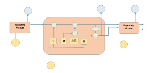
上图在黄色方框中描绘了四个神经网络层，在绿色圆圈中描绘了逐点算子，在黄色圆圈中描绘了输入，在蓝色圆圈中描绘了细胞状态。 LSTM 模块具有一个单元状态和三个门，这为它们提供了有选择地学习、取消学习或保留来自每个单元的信息的能力。 LSTM 中的单元状态通过只允许一些线性交互来帮助信息流过单元而不被改变。 每个单元都有一个输入、输出和一个遗忘门，可以将信息添加或删除到单元状态。 遗忘门使用 sigmoid 函数决定应该忘记来自先前单元状态的哪些信息。 输入门分别使用"sigmoid"和"tanh"的逐点乘法运算控制信息流到当前单元状态。 最后，输出门决定哪些信息应该传递到下一个隐藏状态

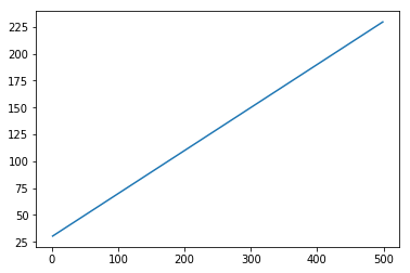
现在我们已经了解了 LSTM 模型的内部工作原理，让我们来实现它。 为了理解 LSTM 的实现，我们先从一个简单的例子 − 一条直线。 让我们看看，LSTM 是否可以学习直线的关系并对其进行预测。

首先让我们创建描绘直线的数据集。

In [402]:

x = numpy.arange (1,500,1)
y = 0.4 * x + 30
plt.plot(x,y)

Out[402]:

[<matplotlib.lines.Line2D at 0x1eab9d3ee10>]

In [403]:

trainx, testx = x[0:int(0.8*(len(x)))], x[int(0.8*(len(x))):]
trainy, testy = y[0:int(0.8*(len(y)))], y[int(0.8*(len(y))):]
train = numpy.array(list(zip(trainx,trainy)))
test = numpy.array(list(zip(trainx,trainy)))

现在数据已经创建并拆分为训练和测试。 让我们根据回溯期的值将时间序列数据转换为监督学习数据的形式，回溯期本质上是在时间"t"处预测值的滞后数。

所以像这样的时间序列 −

time variable_x
t1  x1
t2  x2
 :   :
 :   :
T   xT

当回溯期为 1 时，转换为 −

x1   x2
x2   x3
 :    :
 :    :
xT-1 xT

In [404]:

def create_dataset(n_X, look_back):
   dataX, dataY = [], []
   for i in range(len(n_X)-look_back):
      a = n_X[i:(i+look_back), ]
      dataX.append(a)
      dataY.append(n_X[i + look_back, ])
   return numpy.array(dataX), numpy.array(dataY)

In [405]:

look_back = 1
trainx,trainy = create_dataset(train, look_back)
testx,testy = create_dataset(test, look_back)

trainx = numpy.reshape(trainx, (trainx.shape[0], 1, 2))
testx = numpy.reshape(testx, (testx.shape[0], 1, 2))

现在将训练我们的模型。

将小批量的训练数据显示给网络，将整个训练数据分批显示给模型并计算误差的一次运行称为 epoch。 将运行这些时期，直到错误减少的时间。

In [ ]:

from keras.models import Sequential
from keras.layers import LSTM, Dense

model = Sequential()
model.add(LSTM(256, return_sequences = True, input_shape = (trainx.shape[1], 2)))
model.add(LSTM(128,input_shape = (trainx.shape[1], 2)))
model.add(Dense(2))
model.compile(loss = 'mean_squared_error', optimizer = 'adam')
model.fit(trainx, trainy, epochs = 2000, batch_size = 10, verbose = 2, shuffle = False)
model.save_weights('LSTMBasic1.h5')

In [407]:

model.load_weights('LSTMBasic1.h5')
predict = model.predict(testx)

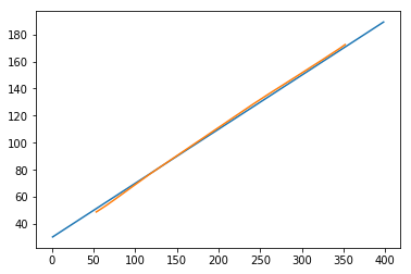
现在让我们看看我们的预测是什么样的。

In [408]:

plt.plot(testx.reshape(398,2)[:,0:1], testx.reshape(398,2)[:,1:2])
plt.plot(predict[:,0:1], predict[:,1:2])

Out[408]:

[<matplotlib.lines.Line2D at 0x1eac792f048>]

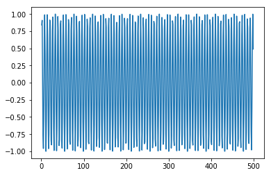
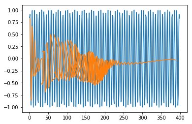
现在，我们应该尝试以类似的方式对正弦波或余弦波进行建模。 您可以运行下面给出的代码并使用模型参数来查看结果如何变化。

In [409]:

x = numpy.arange (1,500,1)
y = numpy.sin(x)
plt.plot(x,y)

Out[409]:

[<matplotlib.lines.Line2D at 0x1eac7a0b3c8>]

In [410]:

trainx, testx = x[0:int(0.8*(len(x)))], x[int(0.8*(len(x))):]
trainy, testy = y[0:int(0.8*(len(y)))], y[int(0.8*(len(y))):]
train = numpy.array(list(zip(trainx,trainy)))
test = numpy.array(list(zip(trainx,trainy)))

In [411]:

look_back = 1
trainx,trainy = create_dataset(train, look_back)
testx,testy = create_dataset(test, look_back)
trainx = numpy.reshape(trainx, (trainx.shape[0], 1, 2))
testx = numpy.reshape(testx, (testx.shape[0], 1, 2))

In [ ]:

model = Sequential()
model.add(LSTM(512, return_sequences = True, input_shape = (trainx.shape[1], 2)))
model.add(LSTM(256,input_shape = (trainx.shape[1], 2)))
model.add(Dense(2))
model.compile(loss = 'mean_squared_error', optimizer = 'adam')
model.fit(trainx, trainy, epochs = 2000, batch_size = 10, verbose = 2, shuffle = False)
model.save_weights('LSTMBasic2.h5')

In [413]:

model.load_weights('LSTMBasic2.h5')
predict = model.predict(testx)

In [415]:

plt.plot(trainx.reshape(398,2)[:,0:1], trainx.reshape(398,2)[:,1:2])
plt.plot(predict[:,0:1], predict[:,1:2])

Out [415]:

[<matplotlib.lines.Line2D at 0x1eac7a1f550>]

Now you are ready to move on to any dataset.